← Alla artiklar Juni 2026 · 30 min · Njurfunktion

Clearance calculation based on a single sample

Jacobssons originalartikel från 1983 om clearance med ett plasmaprov, med mina kommentarer, härledningar och återskapade figurer.

Lars Jacobsson — Department of Radiation Physics, Linköping Hospital, Linköping, Sweden

(Received 19 July 1982; accepted 14 January 1983)

Om denna version. Här återger jag originalartikeln ordagrant i panelerna med seriftext. Mina svenska kommentarer och härledningar står efter respektive avsnitt. Jag har också återskapat figurerna från artikelns formler. Originalfigurerna finns under varje diagram.

Clearance från ett plasmaprov

För att beräkna clearance från ett enda plasmaprov behöver man känna dosen, provtagningstiden och distributionsvolymen. Jacobsson börjar med en förenklad modell och korrigerar sedan för hur spårämnet fördelas i kroppen:

Enkompartmentsmodellen ger $Cl = \frac{V}{t}\ln\frac{Q(0)}{V\,C(t)}$ . Den förutsätter att spårämnet blandas omedelbart och jämnt.
Fördelningen kräver två korrektioner. Innan blandningen är klar hinner extra spårämne elimineras. Det korrigeras med reduktionsfaktorn $r$ . Efter jämvikt är plasmakoncentrationen lägre än medelkoncentrationen i distributionsvolymen. Det korrigeras med $m$ och den effektiva volymen $V' = V/m$ .
Approximation och uppdatering. Både $r$ och $m$ beror på det sökta $Cl$ . Jacobsson ersätter termen $\ln(r)/Cl$ med konstanten $-0{,}0016$ . Beroendet via $m$ finns kvar och hanteras genom att först skatta $Cl$ , sedan uppdatera $m$ och $V'$ och räkna om.

Med formeln undersöker Jacobsson sedan hur fel i $V$ påverkar resultatet och när provet bör tas för att osäkerheten ska bli så liten som möjligt.

Beteckningar

Symbol	Betydelse
$Q(0)$	injicerad mängd/aktivitet (dos)
$Q(t)$	kvarvarande mängd i kroppen vid tid $t$
$\dot{Q}(t)$	utsöndrad mängd per tidsenhet (positiv)
$C(t)$	plasmakoncentration vid tid $t$
$C_0$	extrapolerad koncentration vid $t = 0$
$V$	skattad distributionsvolym
$V'$	effektiv volym i slutformeln, $V/m$
$k$	monoexponentiell eliminationskonstant
$b$	terminal lutning i flerprovsmetoden
$Cl_1$	okorrigerat enkompartments-clearance (“one-pool”)
$r$	reduktionsfaktor för effektiv startdos, $Cl/Cl_1$
$m$	korrektion för icke-uniform distribution

Summary

A formula has been derived for the calculation of renal clearance with the use of a single plasma sample. The formula is based on a one-compartment model. A small correction for non-immediate mixing and non-uniform distribution of the tracer was calculated from empirical data. The accuracy in the calculation method depends on how exactly the distribution volume is known and at what time the blood sample is taken. The expected standard deviation in the clearance value was calculated from data of mean value and spread for the distribution volume of $^{99}\text{Tc}^m\text{-DTPA}$ . In an investigation of 39 subjects with $^{99}\text{Tc}^m\text{-DTPA}$ , a standard deviation of 5 to 6 ml/min was obtained in comparison with a standard method for clearance calculation. This value is in good agreement with the expected one.

Jacobssons formel beräknar njurclearance från ett enda blodprov. Den bygger på en enkompartmentsmodell med två empiriska korrektioner. Noggrannheten beror på hur väl distributionsvolymen är känd och när provet tas. Hos 39 patienter undersökta med ⁹⁹ᵐTc-DTPA var standardavvikelsen i jämförelsen med en etablerad flerprovsmetod 5–6 ml/min, vilket stämde med modellens förutsägelse.

Introduction

It has previously been shown that the tracer concentration in a single plasma sample taken 3-5 h after the injection is correlated to the renal clearance (Tauxe et al., 1971; Fisher & Veall, 1975; Dakubu et al., 1980). Recently, Groth and Aasted (1981) have derived a nomogram and a formula based on a comparison between the tracer concentration in a single sample and the clearance value calculated according to the Bröchner-Mortensen method (1972).

The formula by Groth and Aasted is empirical and not based on any clearance model. In the present communication, a formula is derived from a simple one-compartment model. With this formula it is possible to take into account different distribution volumes correctly and to determine the optimum time for taking the plasma sample. Further, the expected accuracy in the one-sample method can be determined.

Det var redan känt att koncentrationen i ett prov taget 3–5 timmar efter injektionen korrelerar med clearance. Groth & Aasted (1981) hade använt sambandet för att ta fram ett nomogram och en empirisk formel. Jacobsson härleder i stället sin formel ur en fysikalisk modell. Med den kan han ta hänsyn till olika distributionsvolymer, beräkna optimal provtagningstid och uppskatta metodens noggrannhet.

Method

The method is based on a one-compartment model. The distribution volume of the tracer is described by the compartment volume $V$ . The disappearance of the tracer, caused by the renal excretion, is described by a disappearance rate constant $k$ .

Firstly, it is assumed that the tracer is immediately and uniformly mixed in the distribution volume after the injection. After that, a correction for non-immediate mixing is applied and finally the effect of non-uniform distribution is taken into account.

Till att börja med antas spårämnet vara jämnt fördelat i en enda volym $V$ och elimineras med hastighetskonstanten $k$ . Jacobsson korrigerar sedan för att blandningen tar tid och för att plasmakoncentrationen skiljer sig från medelkoncentrationen i hela volymen.

Immediate and Uniform Mixing

According to the definition, the clearance value $Cl$ is given by:

Cl = \frac{\dot{Q}(t)}{C(t)} \quad (1)

where $C(t)$ is the tracer concentration in plasma and $\dot{Q}(t)$ is the excreted amount of tracer per unit time.

Assuming uniform and immediate mixing of the tracer in the volume, the following is valid:

(i) The tracer concentration at any time $t$ is given by:

C(t) = \frac{Q(t)}{V} \quad (2)

where $Q(t)$ is the amount of tracer.

(ii) The disappearance of the tracer is monoexponential from the injection time and the disappearance rate $k = \dot{Q}(t)/Q(t)$ can be written:

k = \frac{1}{t} \ln \left[ \frac{C(0)}{C(t)} \right] \quad (3)

Combining (1) and (2), the clearance value can be written:

Cl = k \times V \quad (4)

and with the use of (3):

Cl = \frac{V}{t} \times \ln \left( \frac{Q(0)}{V \times C(t)} \right) \quad (5)

$Q(0)$ is equivalent to the injected amount of tracer.

Med definitionen av clearance (ekv. 1), jämn och omedelbar blandning (ekv. 2) och exponentiell eliminering (ekv. 3) får man sambandet $Cl = k \times V$ (ekv. 4). Ekv. 5 skriver om det så att clearance kan beräknas från dosen, ett prov och den skattade volymen.

Ekv. 1 — definitionen. Clearance är utsöndrad mängd per tidsenhet delat med plasmakoncentrationen, $Cl = \dot{Q}(t)/C(t)$ . Enheten blir ml/min: volymen plasma som renas helt varje minut. Utsöndras 10 mg/min vid 0,1 mg/ml renas 100 ml/min.
Ekv. 2 — koncentrationen. Om spårämnet är jämnt fördelat i volymen $V$ blir $C(t) = Q(t)/V$ . $V$ är den skenbara distributionsvolymen, inte en anatomiskt avgränsad volym. För DTPA är den typiskt 15–25 liter.
Ekv. 3 — elimineringen. Vid första ordningens kinetik avtar koncentrationen exponentiellt, $C(t) = C(0)\,e^{-kt}$ . Bilda kvoten $C(0)/C(t) = e^{kt}$ , logaritmera och lös för $k$ : $k = \frac{1}{t}\ln[C(0)/C(t)]$ . Konstanten har enheten min⁻¹; halveringstiden är $\ln 2/k$ .
Ekv. 4 — grundsambandet. Sätt in $\dot{Q} = kQ$ (exponentiell eliminering) och $Q = CV$ (ekv. 2) i definitionen: $Cl = kCV/C = k \times V$ . Clearance är alltså produkten av eliminationskonstanten ( $k$ ) och distributionsvolymen ( $V$ ).
Ekv. 5 — enprovsformeln. Byt ut $k$ i ekv. 4 mot uttrycket från ekv. 3 och använd $C(0) = Q(0)/V$ : $Cl = \frac{V}{t}\ln\frac{Q(0)}{V\,C(t)}$ . Beräkningen kräver då dosen $Q(0)$ , ett prov $C(t)$ och en uppskattad volym $V$ . I nästa avsnitt korrigeras antagandena om blandning och fördelning.

Correction for Non-Immediate Mixing

During the first minutes after the injection, before the tracer is completely mixed, the concentration in plasma is greater than during immediate mixing. The greater concentration gives an increased renal excretion which can be interpreted as a loss of tracer activity. The injected amount of tracer, $Q(0)$ in formula (5), therefore shall be reduced by a reduction factor $r$ . The corrected clearance value then can be written:

Cl_r = \frac{V}{t} \times \ln \left( \frac{r \times Q(0)}{V \times C(t)} \right) \quad (6)

Innan spårämnet har blandats färdigt är plasmakoncentrationen högre än modellen förutsätter. Då hinner njurarna eliminera mer spårämne än om dosen hade fördelats jämnt från början. Den extra förlusten finns inte med i den monoexponentiella modellen. Jacobsson räknar därför som om startdosen vore något mindre: med faktorn $r < 1$ ersätts $Q(0)$ av $r \cdot Q(0)$ i ekv. 5. Ju högre clearance, desto mer spårämne hinner elimineras under blandningen och desto lägre blir $r$ .

Correction for Non-Uniform Distribution

After equilibration, when mixing is complete, the tracer concentration is less in plasma than in the distribution volume as a whole (Chantler et al., 1969). The formula (2) therefore shall be modified to:

C(t) = m \times \frac{Q(t)}{V} \quad (7)

where $m$ is a factor less than 1. The factor depends on the clearance value, but is supposed to be constant with time after equilibration. The formulas (4) and (6) then will be altered to:

Cl = k \times V' \quad (8)

and

Cl = \frac{V'}{t} \times \ln \left( \frac{r \times Q(0)}{V' \times C(t)} \right) \quad (9)

where $V' = V/m$ .

Även efter jämvikt är plasmakoncentrationen något lägre än medelkoncentrationen i hela distributionsvolymen, delvis på grund av Gibbs–Donnan-effekten. Om modellen ska använda det uppmätta plasmavärdet som mängd delad med volym måste den effektiva volymen därför vara större. Det uttrycks som $V' = V/m$ med $m < 1$ .

Ekv. 7 — den lägre plasmakoncentrationen. Inför faktorn $m < 1$ : den uppmätta koncentrationen är $C(t) = m\,Q(t)/V$ , alltså bara en andel $m$ av vad enkompartmentsmodellen antog.
Effektiv volym. Skriv om $C = m\,Q/V$ som $C = Q/V'$ . Då blir $V' = V/m$ . Eftersom $m < 1$ är $V' > V$ , typiskt 5–15 % större.
Ekv. 8 och 9 — korrektionen insatt. Sambandet blir $Cl = k\,V'$ (ekv. 8). I ekv. 5 införs sedan båda korrektionerna: $r$ i logaritmens täljare och $V'$ i stället för $V$ (ekv. 9). Både $r$ och $m$ beror dock på $Cl$ , som ännu är okänt. Jacobssons lösning på det kommer längre fram.

Calculation of $r$ and $m$

The factors $r$ and $m$ were calculated by means of two empirical formulas by Bröchner-Mortensen (1980):

Cl = 0.9908 \times Cl_1 - 0.0012 \times Cl_1^2 \quad (10)

and

V_s = \frac{Cl_s}{b} \times \left[ \left( \frac{Cl_s}{Cl_1} \right)^2 - \frac{Cl_s}{Cl_1} + 1 \right] \quad (11)

where $Cl_1$ is clearance calculated from a one pool-system and is given by:

Cl_1 = b \times \frac{Q(0)}{C_0} \quad (12)

where $b$ is the final slope of the plasma curve, $C_0$ is the extrapolated concentration at time 0, $V_s$ is the calculated distribution volume, and $Cl_s$ is clearance according to (10), ' $Cl$ ', with a small correction for different plasma volumes. For a plasma volume of 3000 ml, $Cl_s$ is equal to ' $Cl$ '. In the further calculations, $Cl_s$ has been approximated to ' $Cl$ '.

The reduction factor can be applied on formula (12), which will give a corrected clearance value equal to:

Cl = b \times \frac{r \times Q(0)}{C_0} \quad (13)

The factor $r$ is therefore equal to $Cl/Cl_1$ . By using (10), the factor is obtained as:

r = 0.495 \times (1 + \sqrt{1 - 0.0049 \times Cl}) \quad (14)

The value of $r$ is nearly one for low clearance values and decreases to about 0.8 at high values.

Combining (10) and (11), the distribution volume can be written as:

V = \frac{Cl}{b} \left(0.991 - 0.00122 \times Cl \right) \quad (15)

According to (8) and assuming $k = b$ , the modifying factor is given by:

m = 0.991 - 0.00122 \times Cl \quad (16)

The value of $m$ is nearly one for small clearance values and decreases to about 0.85 at high values.

Här bestämmer Jacobsson $r$ och $m$ med hjälp av Brøchner-Mortensens empiriska samband mellan enkompartmentsvärdet $Cl_1$ och korrigerad clearance.

Beteckningarna skiljer sig mellan artiklarna. Jacobssons $C_0$ och $b$ motsvarar det terminala interceptet $c_1$ och den terminala hastighetskonstanten $b_1$ i Brøchner-Mortensen-artikeln. Där används $C_0$ i kommentaren för startkoncentrationen $Q_0/PV$ , en annan storhet än det terminala interceptet.

Ekv. 10–12 — Brøchner-Mortensens samband. Enkompartmentsvärdet $Cl_1 = b\,Q(0)/C_0$ (ekv. 12) blir för högt eftersom den snabba fördelningsfasen inte räknas med. Ekv. 10 korrigerar värdet: $Cl = 0{,}9908\,Cl_1 - 0{,}0012\,Cl_1^2$ . Korrektionen är liten vid låga värden men växer kvadratiskt (−7 % vid $Cl_1 = 50$ , −19 % vid 150). Ekv. 11 ger motsvarande korrigerade volym.
Ekv. 13–14: $r$ uttryckt i $Cl$ . Division av ekv. 13 med ekv. 12 ger $r = Cl/Cl_1$ . Sätt därefter $Cl_1 = Cl/r$ i ekv. 10 och samla termerna: $r^2 - 0{,}9908\,r + 0{,}0012\,Cl = 0$ . Välj roten som ger $r$ nära 1 vid låg clearance. Med originalets avrundade koefficienter skrivs lösningen $r = 0{,}495\,(1 + \sqrt{1 - 0{,}0049\,Cl})$ . Vid hög clearance sjunker $r$ till omkring 0,8.
Ekv. 15–16: $m$ uttryckt i $Cl$ . Med artikelns approximation $Cl_s \approx Cl$ och $r = Cl/Cl_1$ blir parentesen i ekv. 11 $r^2-r+1$ . Volymsambandet kan då skrivas $V = \frac{Cl}{b}(r^2-r+1)$ . Ekv. 8 ger samtidigt $V = \frac{Cl}{k}m$ ; med $k=b$ följer $m=r^2-r+1$ . Detta är den algebraiska omskrivningen. Därefter approximerar Jacobsson beroendet av $Cl$ med den räta linjen $m \approx 0{,}991-0{,}00122\,Cl$ , vilket ger ekv. 15 och 16.

Clearance Computation

The formulas (14) and (16) cannot be used directly in the calculation of clearance, as $Cl$ is not known in advance. The following procedure therefore has been used for the clearance computation.

Rearranging (9), the clearance value can be written:

Cl = \frac{1}{\frac{t}{V'} - \frac{\ln r}{Cl}} \times \ln \left( \frac{Q(0)}{V' \times C(t)} \right) \quad (17)

The calculated value of the quotient $\ln r/Cl$ is shown as a function of $Cl$ in Fig. 1. The value is nearly constant for $Cl > 20$ ml/min and can, with good approximation, be set equal to $-0.0016$ (ml/min) $^{-1}$ for all clearance values.

The corrected clearance value then can be written:

Cl = \frac{1}{t/V' + 0.0016} \ln \left( \frac{Q(0)}{V' \times C(t)} \right) \quad (18)

The effect of the modifying factor is accounted for by the following procedure: (i) An approximate clearance value, $Cl_r$ , is calculated according to (18) but with the use of the true distribution volume $V$ ; (ii) $m$ is calculated according to (16) with the use of $Cl_r$ ; (iii) The corrected clearance value is calculated according to (18) with the use of $V' = V/m$ .

The error in $Cl$ caused by this procedure is in general less than 1%.

Figur 1. Kvoten ln(r)/Cl beräknad ur ekv. (14). Ovanför Cl ≈ 20 mL/min planar kurvan ut kring den streckade referenslinjen −0,0016 (mL/min)⁻¹ — den approximation som gör att formeln går att lösa.

Visa originalfigur (Jacobsson 1983)

Fig. 1 (original)

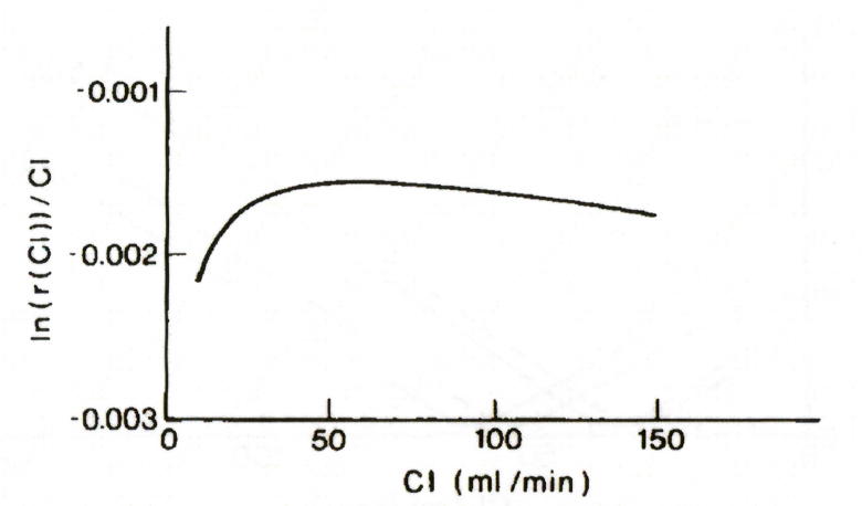
Fig. 1. The quotient ln r/Cl calculated from equation (14).

Jacobsson förenklar termen $\ln r/Cl$ till en konstant. Volymkorrektionen $m$ beräknas däremot från ett preliminärt $Cl$ och används i en ny beräkning.

Ekv. 17: det implicita sambandet. Skriv om ekv. 9 genom att dela logaritmen ( $\ln(r\cdot x) = \ln r + \ln x$ ) och samla $Cl$ . Resultatet innehåller termen $\ln r / Cl$ , så det sökta $Cl$ finns på båda sidor.
Figur 1: approximationen. Ovanför $Cl \approx 20$ ml/min varierar kvoten $\ln r/Cl$ relativt lite kring −0,0016 (ml/min)⁻¹. Jacobsson ersätter därefter termen med denna konstant i huvudformeln för alla clearancevärden.
Ekv. 18: huvudformeln. Approximationen ger $Cl = \frac{1}{t/V' + 0{,}0016}\ln\frac{Q(0)}{V'\,C(t)}$ . Högerledet beror fortfarande på $Cl$ genom $m$ i $V'=V/m$ . Börja med $V'=V$ , beräkna ett preliminärt $Cl$ , uppdatera $m$ och $V'$ och räkna om. Originalet anger att felet från denna uppdatering vanligen är mindre än 1 %. Det avser inte metodens samlade osäkerhet. Uppdateringen används i iohexolverktyget.

Räkneexempel: från ett prov till clearance

En patient väger 70 kg. För ⁹⁹ᵐTc-DTPA blir den skattade volymen $V = 0{,}246 \times 70 \times 1000 = 17\,220$ ml. Ett prov tas $t = 300$ min efter injektionen, och dosen delat med den uppmätta koncentrationen ger $Q(0)/C(t) = 76\,100$ ml.

Varv 0. Börja utan volymkorrektion ( $V' = V$ ):

Cl = \frac{\ln(76\,100/17\,220)}{300/17\,220 + 0{,}0016} = 78{,}1\ \text{ml/min}

Uppdatera: $m = 0{,}991 - 0{,}00122 \times 78{,}1 = 0{,}896$ , alltså $V' = 17\,220/0{,}896 = 19\,225$ ml.

Varv 1. Räkna om med det nya $V'$ :

Cl = \frac{\ln(76\,100/19\,225)}{300/19\,225 + 0{,}0016} = 80{,}0\ \text{ml/min}

Ytterligare en omräkning ändrar svaret mycket lite. Slutvärdet är ≈ 80 ml/min.

Dependence on Error in V

The distribution volume $V$ is dependent on the type of tracer. It has been shown that the volume corresponds to $12.4 \pm 2.4$ (SD) % of body weight ( $m$ ) for inulin (Ladegaard-Pedersen, 1972). For $^{51}\text{Cr-EDTA}$ , the following data has been found: $21.8 \pm 5.1$ (SD) % (Ladegaard-Pedersen, 1971), $20.3 \pm 2.0$ (SD) % for males and $18.8 \pm 2.4$ (SD) % for females (Bröchner-Mortensen, 1980). In this investigation (see clinical application), a value $24.6 \pm 6.9$ (SD) % was found for $^{99}\text{Tc}^m\text{-DTPA}$ . The very large standard deviations found in these investigations implies that the estimation of $V$ for an individual is uncertain with up to 50% variation. However, the calculation of clearance according to (18) is fairly insensitive on the precise value of $V$ , especially if the blood sample is taken at a proper time.

A calculation of clearance using different values of $V$ is shown in Fig. 2. For a clearance value of 100 ml/min and a sample time of 200 min, a 50% error in $V$ will give an error in clearance value of less than 15%.

Cl = 100 mL/minCl = 20 mL/min

t = 200 mint = 300 mint = 500 min

Figur 2. Hur det beräknade clearance-värdet beror på den antagna volymen V, vid sann V = 15 000 mL (lodrät linje). Ju brantare kurva genom skärningspunkten, desto känsligare är svaret för fel i V. Blå kurvor: Cl = 100; gula: Cl = 20. Linjestilen anger provtiden.

Visa originalfigur (Jacobsson 1983)

Fig. 2 (original)

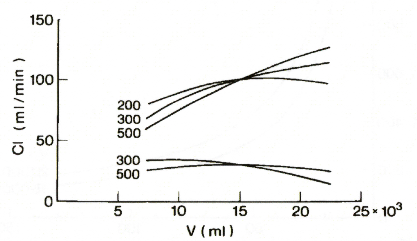
Fig. 2. The dependence of the calculated clearance value, Cl, on the value of the distribution volume, V, for two clearance values, 100 ml/min and 20 ml/min. The curves are valid for the sample time 200, 300 and 500 min after the injection.

Distributionsvolymen $V$ skattas från kroppsvikten, och det är metodens största osäkerhetskälla. I figur 2 är den verkliga volymen $V = 15\,000$ ml. Kurvorna visar hur clearanceberäkningen ändras när ett annat värde på $V$ används. Alla passerar den korrekta punkten. Ju brantare kurvan är där, desto känsligare är resultatet för ett volymfel.

Känsligheten är minst nära den optimala provtiden $t_{opt} = V'/Cl$ . Vid lågt $Cl$ ligger den sent, så ett senare prov hjälper. Vid högt $Cl$ ligger den tidigare, och ett alltför sent prov kan i stället öka känsligheten. Nära optimal provtid ger även ett stort fel i $V$ ett betydligt mindre fel i clearance, som originaltexten ovan beskriver.

The uncertainty in $Cl$ caused by the uncertainty in $V$ was calculated using the above mentioned mean value and standard deviation of $V$ for $^{99}\text{Tc}^m\text{-DTPA}$ . Fig. 3 shows the results of such a calculation made for two different sample times. The calculated standard deviation, $\sigma_{Cl}$ , is thus around 12 ml/min at $Cl = 100$ ml/min and around 4 ml/min at $Cl = 30$ ml/min for a sample time of 300 to 500 min after injection.

t = 300 mint = 500 min

Kroppsvikt 70 kgKroppsvikt 60 kg

Figur 3. Den förväntade standardavvikelsen σ_Cl som osäkerheten i V (24,6 ± 6,9 % av kroppsvikten) ger upphov till, för två kroppsvikter (solid 70 kg, streckad 60 kg) och två provtider (t = 300 och 500 min). Minimum anger det Cl där den valda provtiden sammanfaller med den optimala.

Visa originalfigur (Jacobsson 1983)

Fig. 3 (original)

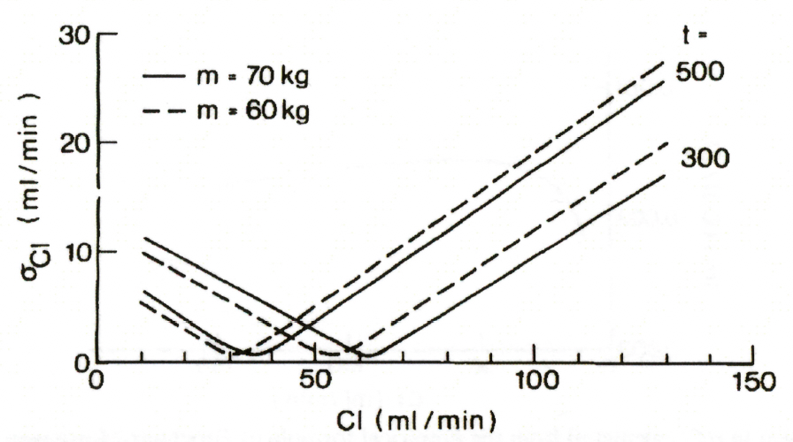
Fig. 3. The expected standard deviation σ_Cl in the clearance value calculated for ⁹⁹ᵐTc-DTPA [V = 24.6 ± 6.9 (SD) % of the body weight 70 kg and 60 kg].

I figur 3 beräknas standardavvikelsen i clearance utifrån hur $V$ varierar mellan individer ( $24{,}6 \pm 6{,}9$ % av kroppsvikten för ⁹⁹ᵐTc-DTPA). Kurvorna visar osäkerheten från volymskattningen. Övriga felkällor ingår inte. För prov vid 300–500 min anges omkring 4 ml/min vid $Cl=30$ och 12 ml/min vid $Cl=100$ . Kurvornas minimum ligger där provtiden är optimal. Därför hjälper ett senare prov vid låg clearance, men inte nödvändigtvis vid hög.

The Optimal Sample Time

The optimal time, $t_{opt}$ , for taking the sample is when the clearance calculation is least dependent on $V$ . This happens when the derivative $dCl/dV'$ of formula (18) is zero, i.e. when $t = V'/Cl$ . Fig. 4 shows $t_{opt}$ as a function of $Cl$ for two distribution volumes $V$ . For clearance values around 100 ml/min, $t_{opt}$ is about 3 h, and for clearance values around 30 ml/min $t_{opt}$ is about 10 h.

V = 15 000 mLV = 20 000 mL

Figur 4. Den optimala provtiden t_opt = V′/Cl, då svaret är minst känsligt för fel i V, för två distributionsvolymer. Den är ungefär medeluppehållstiden och förskjuts till senare tider vid sämre njurfunktion: kring 3 timmar vid Cl = 100, men nästan ett halvt dygn vid mycket låga värden.

Visa originalfigur (Jacobsson 1983)

Fig. 4 (original)

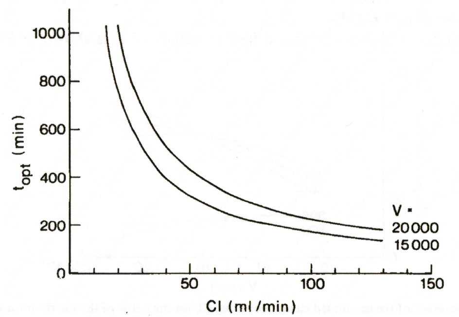
Fig. 4. Optimal time, t_opt, of blood sampling as a function of clearance value for two distribution volumes, 15,000 and 20,000 ml.

Svaret är minst känsligt för fel i $V$ när derivatan $dCl/dV'$ är noll. Det ger den optimala provtiden $t_{opt} = V'/Cl$ , ungefär markörens medeluppehållstid. Ju lägre clearance, desto senare ligger den: omkring 3 timmar vid $Cl = 100$ , men nästan ett halvt dygn vid riktigt låga värden.

Under $Cl = 30$ blir $t_{opt}$ 10 timmar eller mer, vilket sällan är praktiskt genomförbart. Att flytta provet från 4–5 timmar till 8 timmar halverar dock ungefär osäkerheten. I mitt verktyg Optimal provtid (Jacobsson) beräknas $t_{opt}$ från skattad extracellulärvolym och förväntat GFR.

Dependence on Errors in $Q(0)$ and $C(t)$

The error $\Delta Cl$ which appears in $Cl$ for a certain error in $Q(0)$ or $C(t)$ can be written:

\Delta Cl = \frac{1}{t/V' + 0.0016} \times \left( \frac{\Delta Q(0)}{Q(0)} - \frac{\Delta C(t)}{C(t)} \right)

The error is nearly independent on the clearance value. For $V' = 15,000$ ml, a relative error of 10% in $Q(0)$ or $C(t)$ will give errors of 5 ml/min for $t = 300$ min and 3 ml/min for $t = 500$ min.

Uttrycket ovan fås genom att derivera ekv. 18 med avseende på $Q(0)$ och $C(t)$ . Det beskriver hur relativa mätfel påverkar clearance. Minustecknet visar att en för hög uppmätt $C(t)$ ger ett för lågt $Cl$ .

Felet är nästan oberoende av clearancevärdet. Ett 10-procentigt fel i kvoten $Q(0)/C(t)$ , eller i en av variablerna, ger omkring 5 ml/min vid 300 min och 3 ml/min vid 500 min. Om båda mätningarna har oberoende slumpfel kombineras osäkerheterna kvadratiskt. Jacobsson bedömer ±10 % i kvoten som tillräckligt, vilket medger kortare räknetider i gammaräknaren.

Clinical Application

The method was tested on 39 patients, examined with 150 MBq of $^{99}\text{Tc}^m\text{-DTPA}$ . Four blood samples were drawn 240, 260, 280 and 300 min after the injection. One millilitre of plasma from each sample was measured in a gamma well counter for 1 min on the day after the examination. From the activity concentration in the four samples, clearance was calculated according to the Bröchner-Mortensen method (1972). The final slope $b$ of the plasma curve was obtained by the least squares method and the ‘one-pool clearance’, $Cl_1$ , was calculated from formula (12). The corrected clearance value was calculated according to formula (10). Clearance, according to the one-sample method [formula (18)] was calculated for the 240 and 300 min samples. The distribution volume used in the calculation was 24.6% of the body mass. This value was obtained as the mean value of the calculated distribution volumes [formula (11)] for the 39 patients.

Fig. 5 shows the comparison between clearance values obtained with the Bröchner-Mortensen method and the one-sample method with the sample time $t = 300$ min. The mean difference between the two values was $2.3 \pm 1.0$ (SEM) ml/min and the standard deviation was 6.1 ml/min. The mean difference between the clearance values calculated from the Bröchner-Mortensen method and the 240 min sample was $2.4 \pm 0.8$ (SEM) ml/min and the standard deviation was 5.3 ml/min.

Fig. 5

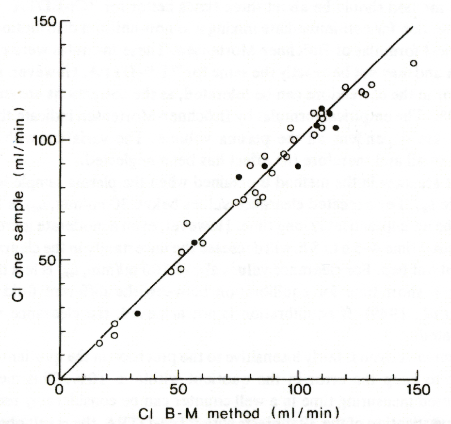
Fig. 5. Comparison of clearance calculated with the Bröchner-Mortensen method and with the one-sample method (sample time 300 min). The investigation was made with ⁹⁹ᵐTc-DTPA. ○ = Solco nuclear, ● = Cea Ire Sorin.

Enprovsmetoden (ekv. 18) jämfördes med Brøchner-Mortensens flerprovsberäkning hos 39 patienter. För provet vid 300 minuter var medelavvikelsen 2,3 ml/min och standardavvikelsen för skillnaderna 6,1 ml/min. Det är den observerade spridningen mellan metoderna. Figur 3 visar i stället den osäkerhet som modellen förutsäger från variationen i $V$ . Jacobsson bedömde att resultaten stämde väl överens. Volymskattningen 24,6 % av kroppsvikten kommer från samma 39 personer.

Discussion

The formula derived for clearance determination with one sample requires that the distribution volume, $V$ , is known. The accuracy in the estimation of $V$ for an individual determines the accuracy in the method. In this investigation, a great spread was found in the quotient $V/m$ for $^{99}\text{Tc}^m\text{-DTPA}$ compared to an investigation with $^{51}\text{Cr-EDTA}$ (Bröchner-Mortensen, 1980). If the difference in spread is real, the accuracy in the one-sample method should be about three times better for $^{51}\text{Cr-EDTA}$ .

The correction for non-immediate mixing and non-uniform distribution are derived from empirical formulas of Bröchner-Mortensen. These formulas were calculated for $^{51}\text{Cr-EDTA}$ and may not be exactly the same for $^{99}\text{Tc}^m\text{-DTPA}$ . However, a rather great relative error in the corrections can be tolerated, as the corrections are small, typically less than 10%. The empirical formulas by Bröchner-Mortensen indicate that the values of $r$ and $m$ are dependent on the plasma volume. The variation with the volume, however, is small and therefore the effect has been neglected.

The best accuracy in the method is obtained when the plasma sample is taken at the optimal time $t_{opt}$ . For expected clearance values below 30 ml/min, $t_{opt}$ is 10 h or more which may be an impracticably long time. However, even a moderate increase from the commonly used time 4-5 h to 8 h, will decrease the uncertainty in the clearance value by a factor of about two. For clearance values above 100 ml/min, $t_{opt}$ is less than 2 h. This may be a too short time for equilibration between the different fluid components (Chantler et al., 1969). If equilibration is not achieved, the clearance value will be underestimated.

The formula derived is fairly insensitive to the precision in the quotient $Q(0)/C(t)$ . It is sufficient to keep the error in the quotient within $\pm 10\%$ . This means that the commonly used measuring time in a well counter can be considerably reduced.

In the investigation of the 39 subjects with $^{99}\text{Tc}^m\text{-DTPA}$ , the result obtained at high clearance values is somewhat better than the predicted one. At low clearance values the accuracy also seems to be at least as good as the predicted one, for the few subjects examined. However, further investigations are needed, with blood sampling at the later time of 8 h or more after the injection to control the reliability of the method at low clearance values.

In summary, the derived formula is useful in calculating clearance using a single sample drawn at any time after the equilibration. Accuracy in the calculation will be improved when a more exact distribution volume is known and with the sample being drawn nearer to the optimal time.

Hur väl $V$ är känt har störst betydelse för noggrannheten. Spridningen i $V/m$ var stor för ⁹⁹ᵐTc-DTPA. För ⁵¹Cr-EDTA, där spridningen är mindre, bedömde Jacobsson att metoden borde bli ungefär tre gånger noggrannare.

Korrektionerna $r$ och $m$ är typiskt under omkring 10 % vid låg clearance, men 10–20 % eller mer vid hög. Osäkerheten i korrektionerna påverkar resultatet mindre än osäkerheten i $V$ , och därför tolereras relativt stora fel i dem. Beroendet av plasmavolymen kan också försummas.

Provet bör tas nära $t_{opt}$ . Vid hög clearance blir tiden dock < 2 timmar, och då kan spårämnet ännu inte ha nått jämvikt. Clearance underskattas i så fall. Formeln kan användas efter jämvikt, med bättre noggrannhet ju närmare optimal provtid provet tas och ju bättre distributionsvolymen är känd.

Osäkerhet och provtid

Tre typer av fel påverkar beräkningen:

Modellfel. Enkompartmentsmodellen förenklar både blandningen och fördelningen. Faktorerna $r$ och $m$ korrigerar delvis för detta.
Fel i $V$ . Den verkliga distributionsvolymen kan avvika från den viktbaserade skattningen. Detta är oftast den största felkällan.
Mätfel i $Q(0)/C(t)$ . Hit hör doskalibrering, provmätning och räkneprecision. Beräkningen är relativt okänslig för dessa fel; Jacobsson anger ±10 % som tillräcklig noggrannhet i kvoten.

Eftersom fel i $V$ brukar dominera bör provet tas så nära $t_{opt} = V'/Cl$ som praktiskt möjligt. Vid låg clearance innebär det ofta senare provtagning än de vanliga 4–5 timmarna.

Iohexolkalkylator

Korrektionerna i beräkningen

I verktygets enprovsberäkning används följande korrektioner och uppdatering:

m, volymkorrektionen. Efter jämvikt är plasmakoncentrationen något lägre än genomsnittet i distributionsvolymen. Den motsvarar därför en effektiv volym $V' = V/m$ , större än $V$ eftersom $m < 1$ . Faktorn approximeras empiriskt: $m = 0{,}991 - 0{,}00122 \times Cl$ .
r, reduktionsfaktorn för tidig förlust. Innan spårämnet blandats färdigt är plasmakoncentrationen förhöjd, vilket ger extra tidig renal elimination. Den effektiva startdosen skrivs $r \cdot Q(0)$ , där $r = Cl/Cl_1 < 1$ , och approximeras med $r = 0{,}495 \times (1 + \sqrt{1 - 0{,}0049 \times Cl})$ .
Iterationen. Börja med $V' = V$ och beräkna ett preliminärt $Cl$ med ekv. 18. Beräkna sedan $m = 0{,}991 - 0{,}00122 \times Cl$ , sätt $V' = V/m$ och räkna om $Cl$ . I ekv. 18 uppdateras bara $m$ och $V'$ , eftersom effekten av $r$ redan ingår i konstanten $0{,}0016$ . En iteration räcker oftast för klinisk noggrannhet; full konvergens nås inom några varv.

Jag använder samma beräkning i mitt iohexolverktyg. Där kan du ange patientdata och provsvar, beräkna clearance med Jacobsson-iterationen och se koncentration–tid-kurvan och delberäkningarna.

References

BRÖCHNER-MORTENSEN J. (1972) A simple method for the determination of glomerular filtration rate. Scand. J clin Lab Invest, 30, 271-274.
BRÖCHNER-MORTENSEN J. (1980) A simple single injection method for determination of the extracellular fluid volume. Scand J clin Lab Invest, 40, 567-573.
CHANTLER C., GARNETT S. E., PARSONS V. & VEALL N. (1969) Glomerular filtration rate measurement in man by the single injection method using $^{51}\text{Cr-EDTA}$ . Clin Sci, 37, 169-180.
DAKUBU S., ADU D., NKRUMAH K. N., ANIM-ADDO Y. & BELCHER E. H. (1980) Single blood sample estimation of glomerular filtration rate. Nucl Med Comm, 1, 83-86.
FISHER M. & VEALL N. (1975) Glomerular filtration rate estimation based on a single blood sample. Br Med J, 2, 542.
GRANERUS G. & JACOBSSON L. (1985) Calculation of $^{51}\text{Cr-EDTA}$ single injection clearance. Comparison between a single sample and multiple sample formula. Swedish Soc Radiol Proc, 19, 71-73.
GROTH S. & AASTED M. (1981) $^{51}\text{Cr-EDTA}$ clearance determined by one plasma sample. Clin Physiol, 1, 417-425.
LADEGAARD-PEDERSEN H. J. & ENGELL H. C. (1972) A comparison of distribution volumes of inulin and $^{51}\text{Cr-EDTA}$ in man and nephrectomized dogs. Scand J clin Lab Invest, 30, 267-270.
TAUXE W. N., MAHER F. T. & TAYLOR W. F. (1971) Effective renal plasma flow: estimation from theoretical volumes of distribution of intravenously injected $^{131}\text{I-orthoiodohippurate}$ . Mayo Clin Proc, 46, 524-531.

Jacobsson L. (1983). A method for the calculation of renal clearance based on a single plasma sample. Clinical Physiology, 3(4), 297–305. Originalförfattare: Lars Jacobsson, Avdelningen för radiofysik, Linköpings lasarett. Kommentarer, härledningar och återskapade figurer är tillägg till originalartikeln.

Clearance calculation based on a single sample

Summary

Introduction

Method

Immediate and Uniform Mixing

Correction for Non-Immediate Mixing

Correction for Non-Uniform Distribution

Calculation of rrr and mmm

Clearance Computation

Dependence on Error in V

The Optimal Sample Time

Dependence on Errors in Q(0)Q(0)Q(0) and C(t)C(t)C(t)

Clinical Application

Discussion

Iohexolkalkylator

References

Calculation of $r$ and $m$

Dependence on Errors in $Q(0)$ and $C(t)$